FyDiK documentation

FyDiK = Fyzikální Diskretizace Kontinua
Physical Discretization of Continuum
November 2009, Petr Frantík
last update: March 2011
http://www.kitnarf.cz

FyDiK documentation (version 3.26 and later)
Petr Frantík

Introduction
Terms
Application execution
Data files
Basic objects and functional units
Mass point
Translational spring
Rotational spring
Numerical solution
Notes
References

Introduction

The application FyDiK serves for interactive simulation of a nonlinear dynamical system which is representation of a mechanical structure. It is possible to use it for calculation of vibrations of a structure, strain and stress analysis, large deflections of beams, full scale stability analysis, material damage and fracture, etc. Solving and visualizing is provided numerically in real-time and can be controlled by user. Application allows full nonlinearity, state of all objects can be simultaneously saved and numerical model can be changed on the fly.

Terms

Boundary conditions: are time independent conditions for values of state variables of the system, which the dynamical system has to satisfy.
Dynamical system: is formal name for a set of rules which describes the time dependence of a point's position in the state space of the system, see also. In the application FyDiK these rules namely correspond with the second Newton's law.
Initial conditions: are conditions for values of state variables of the system, which the dynamical system has satisfy in a particular time. In the application FyDiK in zero time.
Nonlinear behaviour: means that the change of the system initial conditions is not proportional to the change of the system solution. Generally typical nonlinear phenomenons exist like jumps, bifurcations, deterministic chaos, see also.
Simulation: serves for discovering of time evolution of the dynamical system from the specific initial conditions.
State variables: are variable numbers (functions) which describes the current system state in time. The system state is totally defined by them. These variables correspond with coordinates of a point in the state space of the system. In the application FyDiK this means namely coordinates and current velocities of all mass points.
State space: is a virtual space in which every point corresponds with unique system state. Point's coordinates are state variables of the system. The system dimension is therefore necessarily equal to the number of state variables. In the state space the evolving system develops continuous trajectory.
Trajectory of the system: is representation of the solution of the dynamical system in its state space. It is continuous curve which represents the time evolution of the system. The trajectory cannot cross itself due to the requirement of the unambiguous evolution, see also.

Application execution

In order to the execution of the FyDiK application, there has to be a Java platform installed in operating system. The platform can be downloaded from http://www.java.com/en/download/manual.jsp. If the Java platform is installed properly the application JAR file fydik2dapplication.jar can be executed.

The application FyDiK is possible to execute directly (by click on fydik2dapplication.jar) or from the operating system command line (if the system offers it). The command line execution is well suitable for batch processing or for viewing of detailed warnings or exceptions. The execution will be provided by entering the following string to the command line (if we are in the directory where file fydik2dapplication.jar is presented):

java -jar fydik2dapplication.jar

or more in detail:

java -jar fydik2dapplication.jar -projectName [name] -directoryName [path]

where [name] is the project name and [path] is the path to the project directory. For example let's have the file fydik2dapplication.jar and subdirectory data in the directory C:/fydik. And in the subdirectory data a project bridge (files bridge.model.fdk and bridge.settings.fdk). Then execution string will have following form:

java -jar fydik2dapplication.jar -projectName bridge -directoryName data

Used directory separator is platform dependent.

Data files

A FyDiK application project consists from two XML data files labelled model and settings. As name leads, the model file defines objects of dynamical system and parameters of simulator. The settings file contains parameters of GUI (graphic user interface). There is an example of XML structure of model data file:

Such data file can be easy generated, edited and fixed.

Basic objects and functional units

FyDiK2D model is designed for simple and clear physical representation and functionality. On fig. 1 two basic functional units are shown: normal unit and bending unit, composed from three basic model objects. The normal unit originates by connection of two mass points with translational spring. The bending unit originates by connection of two translational springs by rotational spring. A translational spring allows forced normal displacement of the normal unit and a rotational spring allows forced bending displacement of the bending unit.


normal unit	bending unit

Fig. 1: Basic functional units (top physical representation, bottom FyDiK application representation)

Each of three objects can be from the implementation point of view understand as an object in the sense of object oriented programming (see), e.g. it has attributes, state variables and methods.

Mass point (class MassPoint)

Mass point is key object of the model. It is chosen to carry the mass. Its state is given by state variables, which are coordinates x_i, y_i and velocity components v_xi, v_yi. Mass point can be also understands as a mass hinge, because it transmits forces between two connected translational springs and this term represents well its physical functionality.

Set of coordinates and velocity components of every mass point define majority of all state variables of the model. Mass points are targets of force loading by reason of accumulation of the mass. It can be imagined that the other objects serve for loading of them only.

Fig. 2: Mass point in the plane with cartezian coordinate system and its state variables

On fig. 2 a mass point is shown with index i including cartezian coordinate system and its state variables.

Every mass point has following attributes: standalone mass m_0i, initial conditions x_i(0)=x_0i, y_i(0)=y_0i, v_xi(0)=v_x0i, v_yi(0)=v_y0i, boundary conditions (e.g. fixed value of a coordinate or a velocity component) and function of viscose damping. Function of viscose damping defines size of damping force F_di:

$\vec{F}_{di}=-c_i \vec{v_i} (1+c_{2i}|\vec{v_i}|+c_{3i}|\vec{v_i}|^2),$

(1)

where v_i is vector of mass point velocity, c_i, c_2i, c_3i are given coefficients. The damping force is named as constant, according to size of mass m_i. Its alternative named proportional means that force given by equation (1) is multiplied by size of mass m_i.

As was mentioned, mass points are key objects of the dynamical system. The dynamical system can be now written in the following form:

$\begin{array}{l} \displaystyle \frac{\mbox{d}x_i}{\mbox{d}t} = v_{xi}, \;\; \frac{\mbox{d}v_{xi}}{\mbox{d}t} = \frac{1}{m_i}(R_{xi}+F_{dxi}), \\ \\ \displaystyle \frac{\mbox{d}y_i}{\mbox{d}t} = v_{yi}, \;\; \frac{\mbox{d}v_{yi}}{\mbox{d}t} = \frac{1}{m_i}(R_{yi}+F_{dyi}), \end{array} ,$

(2)

where m_i is current mass of the mass point, which is the sum of standalone mass m_0i and masses distributed from connected objects (e.g. from a translational spring). Symbols R_xi, R_yi means vector components of force resultant by which other objects loads the mass point, F_dxi, F_dyi are components of damping force and t is time.

Translational spring (class TranslationalSpring)

Translational spring ensures connection of two mass points. Physical representation of a translational spring is a light and rigid telescopic bar with inner spring, see fig. 3. This spring loads both connected mass points by defined interaction force F_tij of the size given by arbitrary defined function dependent on spring elongation Δl_ij. The orientation of the force is the same as orientation of the spring.

Fig. 3: Translational spring and its angle

Translational spring has following basic attributes: reference length l_ij, initial angle counter c_φ0ij (an integer number implicitly set to zero), references on two mass points, interaction function F_tij(Δl_ij) and damping function given by the same way as for a mass point. Additionally the spring has following optional attributes for user comfort: volume density ρ_ij and area of cross-section A_ij, from which the mass of the spring can be calculated and numerically distributed to the connected mass points.

Note that reference length of the spring l_ij can be in the application specified by a value or by initial or actual state of the dynamical system.

For spring elongation Δl_ij following applies:

$\Delta l_{ij}=l_{aij}-l_{ij}, \,\,\, l_{aij}=\sqrt{(x_j-x_i)^2+(y_j-y_i)^2},$

(3)

where l_aij is the current length of the spring.

Translational spring has one state variable: the angle counter c_φij which helps to define its absolute rotation φ_aij. This variable is necessary due to requirement of calculation of rotation larger than 2π or smaller than zero. This necessity is in relation with definition of the rotational spring as will be described later. Coordinates of connected mass points can be in this sense used for calculation of constrained angle φ_sij from interval (0,2π) by relationship:

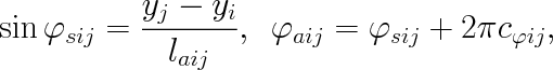$\sin \varphi_{sij}=\frac{y_j-y_i}{l_{aij}}, \,\,\, \varphi_{aij}=\varphi_{sij}+2 \pi c_{\varphi ij},$

(4)

where actual angle counter c_φij is an integer number, which remain constant if change of the constrained angle φ_sij is in absolute values smaller than π. In the case when the change is larger than π the single increment is made according to the sign of value of change. This procedure enables possibility to consistently calculate arbitrary rotation of the spring.

Translational spring can be damped. Damping force has the same form as for mass points, see equation (1), but velocity in this equation is relative velocity of the second mass point according to the first mass point in the angle of the spring. Therefore this damping is acting only if the spring is changing its length.

Rotational spring (class RotationalSpring)

Rotational spring ensures bending connection of two translational springs. Physical representation of a rotational spring is thin coiled elastic plate (e.g. spring inside mechanical watches) or elastic band around the hinge, which makes connection of two translational springs, see fig. 4. The rotational spring loads translational springs by moment M_rijk, which size is given by a function dependent on rotation of the rotational spring Δφ_ijk. The moment M_rijk produces two couples of forces F_rij and F_rjk, which loads mass points i, j and k. These forces act perpendicularly to translational springs.

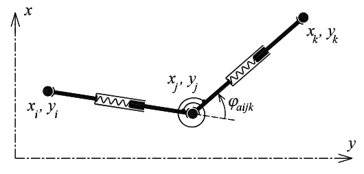
Fig. 4: Rotational spring

Rotational spring has following basic attributes: reference angle φ_ijk, references on two translational springs, interaction function M_rijk(Δφ_ijk) and damping function given by the same way as for a mass point and translational spring. Additionally the spring has following optional attributes for user comfort: mass m_rijk and cross-section modulus W_ijk. The modulus serves for calculation of normal stress, which is useful for monitoring of extreme stress of bended beams.

Note that reference angle φ_ijk can be in the application specified by a value or by initial or actual state of the dynamical system (similarly as the reference length for a translational spring).

For rotation Δφ_ijk of the spring applies:

$\Delta \varphi_{ijk}=\varphi_{aijk}-\varphi_{ijk}, \,\,\, \varphi_{aijk}=\varphi_{ajk}-\varphi_{aij},$

(5)

where φ_aijk is current angle between referenced translational springs -- difference between their current angles φ_aij and φ_ajk.

Rotational spring has no state variable. Its state is unambiguously given by its attributes and by state of referenced translational springs.

Also rotational spring can be damped. Damping function has similar form as for mass points, see equation (1), but it is adopted for rotation into following relationship:

$M_{dijk}=-c_{ijk}\,\omega_{ijk} (1+c_{2ijk}\,|\omega_{ijk}|+c_{3ijk}\,\omega_{ijk}^2),$

(6)

where M_dijk is damping moment, which acts the same way as moment M_rijk, ω_ijk is current relative angular velocity between referenced translational springs -- difference between their current angular velocities ω_ij and ω_jk.

Numerical solution

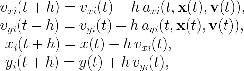
Dynamical system, its main equations (2) were described early, is solved in the application by numerical methods for solving ordinary differential equation with a given initial value. Particularly by explicit Euler method, modified explicit Euler method and by classical Runge-Kutta method (fourth order). The simplest Euler method solve equation system (2) as follows:

$\begin{array}{l} v_{xi}(t+h)=v_{xi}(t)+h\,a_{xi}(t,\mathbf{x}(t),\mathbf{v}(t)), \\ v_{yi}(t+h)=v_{yi}(t)+h\,a_{yi}(t,\mathbf{x}(t),\mathbf{v}(t)), \\ \,\,x_i(t+h)=x(t)+h\,v_{xi}(t), \\ \,\,y_i(t+h)=y(t)+h\,v_{y_i}(t), \end{array}$

(7)

where h is numerical step, functions of acceleration a are equal to right sides of equations of the dynamical system (2) and x, v represents all state variables. You can see that for calculation of new state is only neccessary to know values for previous state. This method is stable only for very small step and practically it is unusable.

Better results can be obtained by tiny modification of Euler method. Simply use velocities of the new state for calculation of new coordinates:

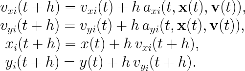$\begin{array}{l} v_{xi}(t+h)=v_{xi}(t)+h\,a_{xi}(t,\mathbf{x}(t),\mathbf{v}(t)), \\ v_{yi}(t+h)=v_{yi}(t)+h\,a_{yi}(t,\mathbf{x}(t),\mathbf{v}(t)), \\ \,\,x_i(t+h)=x(t)+h\,v_{xi}(t+h), \\ \,\,y_i(t+h)=y(t)+h\,v_{y_i}(t+h). \end{array}$

(8)

Classical Runge-Kutta method is more complicated. It gives more reliable results. See reference for more informations.

Notes

The homepage of the FyDiK application is http://fydik.kitnarf.cz.

References

Macur, J.: Dynamické systémy, http://www.fce.vutbr.cz/studium/materialy/Dynsys

Wikipedia, the free encyclopedia: Dynamical system, http://en.wikipedia.org

Wikipedia, the free encyclopedia: Euler method, http://en.wikipedia.org

Wikipedia, the free encyclopedia: Nonlinear system, http://en.wikipedia.org

Wikipedia, the free encyclopedia: Ordinary differential equation, http://en.wikipedia.org

Wikipedia, the free encyclopedia: Runge-Kutta method, http://en.wikipedia.org